Pricing Model & Implied Volatility

This section presents the mathematical framework for pricing Timelock positions by equating option premia with liquidity provider fee collection, ultimately deriving implied volatility from Uniswap market data.

Pricing Mechanisms Overview

Pricing can be implemented using multiple approaches:

1. Standard Black Scholes Model Option Price - taking IV off-chain and price on-chain
2. Standard Black Scholes Model Option Price - taking IV and price both derived from the pool
3. Multiple of Swap fees forward calculated - not timed
4. Borrowing Rate forward calculated - not timed

Premium Pricing

This is a new derivative which does not have a predefined pricing mechanism. However, it bears close resemblance to an ATM call long or a future long+ put position.

Standard Black-Scholes-Merton Model

The standard pricing mechanism for a call option is given by the Black-Scholes-Merton model as:

$$C = N(d_1)S_t - N(d_2)Ke^{-rt}$$

Where:

$$d_1 = \frac{\ln\left(\frac{S_t}{K}\right) + \left(r + \frac{\sigma^2}{2}\right)t}{\sigma\sqrt{t}} \quad \text{and} \quad d_2 = d_1 - \sigma\sqrt{t}$$

Parameters:

• $C$ = call option price
• $N$ = CDF of the normal distribution
• $S_t$ = spot price of an asset
• $K$ = strike price
• $r$ = risk-free interest rate
• $t$ = time to maturity
• $\sigma$ = volatility of the asset

ATM Call Option Adaptation

In an ATM call option, $K = S_t$, so $d_1$ and $d_2$ become:

$$d_1 = \frac{\left(r + \frac{\sigma^2}{2}\right)t}{\sigma\sqrt{t}}$$ $$d_2 = d_1 - \sigma\sqrt{t} = \frac{\left(r + \frac{\sigma^2}{2}\right)t}{\sigma\sqrt{t}} - \sigma\sqrt{t} = \frac{rt}{\sigma\sqrt{t}}$$

The pricing formula becomes:

$$C(S_t, t) = S_t \cdot N\left(\frac{\left(r + \frac{\sigma^2}{2}\right)t}{\sigma\sqrt{t}}\right) - S_t \cdot e^{-rt} \cdot N\left(\frac{-rt}{\sigma\sqrt{t}}\right)$$

Crypto Asset Adaptation (r = 0)

For crypto assets, we use risk-free rate $r = 0$, so the formula simplifies to:

For $d_1$ and $d_2$ with $r = 0$:

$$d_1 = \frac{\left(0 + \frac{\sigma^2}{2}\right)t}{\sigma\sqrt{t}} = \frac{\sigma\sqrt{t}}{2}$$ $$d_2 = d_1 - \sigma\sqrt{t} = \frac{\sigma\sqrt{t}}{2} - \sigma\sqrt{t} = -\frac{\sigma\sqrt{t}}{2}$$

Final simplified formula:

$$C(S_t, t) = S_t \cdot \left(N\left(\frac{\sigma\sqrt{t}}{2}\right) - N\left(\frac{-\sigma\sqrt{t}}{2}\right) - 1\right)$$

Pool Utilization Optimization

We introduce optimization that accounts for pool utilization to accurately reflect market dynamics. This approach is inspired by peer-to-pool mechanism protocols, most notably AAVE.

Utilization Rate Definition

$$U = \frac{\text{Assets utilized (locked())}}{\text{Total Assets (locked() + free())}}$$

Where:

• $U$ = utilization rate of the pool
• $U_{\text{optimal}}$ = variable rate parameter (optimal utilization threshold)

Premium Calculation Based on Utilization

If $U < U_{\text{optimal}}$:

$$\text{premium} = C(S_t, t)$$

If $U > U_{\text{optimal}}$:

$$\text{premium} = C(S_t, t) + \frac{(U - U_{\text{optimal}}) \cdot C(S_t, t)}{1 - U}$$

Implied Volatility Calculation

Daily Return Calculation

Calculate the daily return of an asset where $P_t$ is the close price at day $t$:

$$\text{Daily Return} = \ln\left(\frac{P_t}{P_{t-1}}\right)$$

Statistical Measures

Mean of Daily Returns:

$$\mu = \frac{1}{N} \sum_{t=1}^{N} \text{Daily Return}_t$$

Variance of Daily Returns:

$$\text{Variance} = \frac{1}{N-1} \sum_{t=1}^{N} (\text{Daily Return}_t - \mu)^2$$

Standard Deviation (Sigma):

$$\sigma = \sqrt{\text{Variance}}$$

Annualized Volatility (Implied Volatility)

$$\text{Annualized Volatility (Implied Volatility)} = \sigma_{\text{daily returns}} \times \sqrt{365}$$

Step 1: Collected Fees from Liquidity Provision

In order to calculate the fees collected from a Uniswap LP position, we consider the total liquidity amount deployed at a given tick.

We have the following:

• Total fees accumulated:

  $$\text{feeRate} \times \text{(volume per day)}$$

  Where feeRate is the percentage fee that spot traders on Uniswap pay when they execute a trade.

• Fraction of those fees that goes to that LP position of size positionSize:

  $$\frac{\text{positionSize}}{\text{tickLiquidity}}$$

  Here, the position size corresponds to the amount of liquidity a liquidity provider (LP) allocates within a specific price range in the liquidity pool.

• Finally, we get:

  $$\text{Total fees at a given tick} = \frac{\text{feeRate} \times \text{(volume per day)} \times \text{positionSize}}{\text{tickLiquidity}}$$

Step 2: Cumulative Premia Using Theta

The cumulative premia is the integral of theta over the asset's price path $S(t)$:

$$\text{Cumulative Premia} = \int S(t) \theta(S_t, K, \sigma) dt = \int_{+\infty}^{0} \theta(S_{\Delta t}, K, \sigma) \Delta t dS_{\Delta t}$$

Where theta ($\theta$) for an option (assuming a zero interest rate and no dividends) is given by:

$$\theta = -\frac{dV(S_t, t)}{dt} = \frac{S \sigma}{\sqrt{8\pi t}} \exp \left(-\frac{[\ln(\frac{S_t}{K}) + \frac{\sigma^2 t}{2}]^2}{2 \sigma^2 t}\right)$$

Step 3: Approximating Theta Using The Dirac Distribution

The Dirac Distribution

The Dirac function, denoted by $\delta(x)$, is a "pseudo-function" that has the following characteristics:

$$\delta(x) = \begin{cases} +\infty & \text{if } x = 0 \\ 0 & \text{otherwise} \end{cases}$$

and

$$\int_{R} \delta(x) dx = 1$$

The graph of $\delta(x)$ can therefore be represented by the entire x-axis and the positive half of the y-axis. With the "Dirac" $\delta(x)$, we aim to represent an impulse or (infinitely short) point event with finite, non-zero "energy".

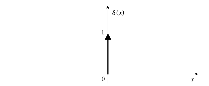
Figure 1: Graph of the Dirac distribution $δ(x)$.

Important Definition/Theorem (See Appendix 3.2): The Dirac function can also be perceived as the limit, as $a$ tends to 0, of the following centered Gaussian function:

$$\frac{1}{a} e^{-(x/a)^2}.$$

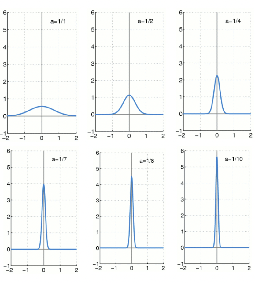
Figure 2: Approximation of the Dirac delta function using different zero-centered normal distributions.

Example: One function commonly used to represent a Dirac delta function is $\delta_p(x) = p \cdot \text{rect}(px)$, where:

$$\text{rect}(px) = \begin{cases} 1 & \text{for } |x| \leq \frac{1}{2p} \\ 0 & \text{otherwise} \end{cases}$$

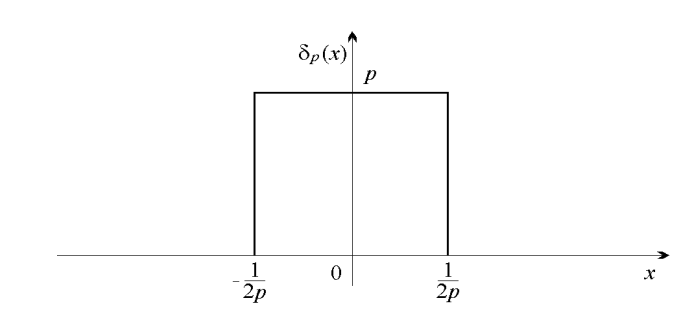
Figure 3: Example of Dirac delta function: Graph of the function $δ_p(x) = p rect(px)$

Comparing the Dirac Function to Theta

We aim to approximate the theta function of options by using an approximation of the Dirac function. The Dirac function increasingly resembles the theta function for options as the days to expiration (DTE) approaches 0. The figure below shows the theta of an option as a function of spot price movements for various DTEs: 7 DTE, 1 DTE, and 0.1 DTE.

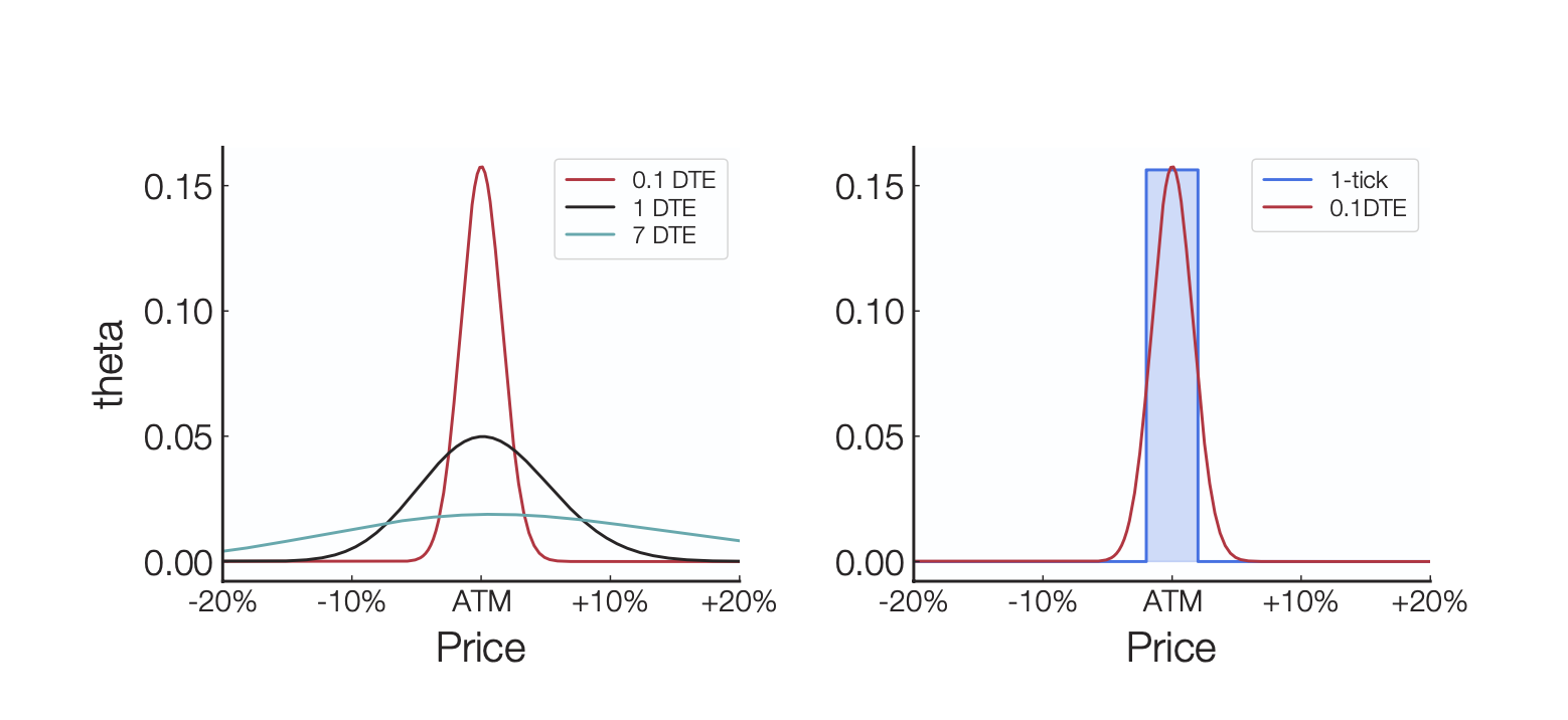
Figure 4: Graph illustrating the variations in theta across different days until expiration.

To understand how this theta can have a limit resembling a Dirac delta function as $t \to 0$, we analyze the components of the two expressions: the theta function and the Dirac delta function:

1. The Dirac delta function, $\delta(x)$, is defined such that:

   $$\delta(x) = \lim_{\epsilon \to 0} \frac{1}{\epsilon \sqrt{2\pi}} \exp \left( - \frac{x^2}{2\epsilon^2} \right).$$

2. The given equation for theta is:

   $$\theta = \frac{S \sigma}{\sqrt{8\pi t}} \exp \left( - \frac{[\ln(\frac{S}{K}) + \frac{\sigma^2 t}{2}]^2}{2 \sigma^2 t} \right).$$

3. We have $A(t) := \frac{[\ln( \frac{S}{K}) + \sigma^2 t / 2]^2}{2 \sigma^2 t}.$

4. Set $x := \ln \left( \frac{S}{K} \right)$ and $\epsilon^2 := \sigma^2 t$. Then,

   $$\theta \approx_{t \to 0} K \cdot e^{x \sigma^2 / 2 \epsilon \sqrt{2\pi}} \exp \left( - \frac{x^2}{2 \epsilon^2} \right).$$

5. Setting the limit: As $t \to 0$, the function $\theta$ approximates a Dirac delta function centered at $S_t = K$ as seen in Figure 4:

   $$\theta \approx_{t \to 0} K \cdot e^{x \sigma^2 / 2} \delta(x).$$

6. We need to make sure that this resulting limit is a Dirac delta function, in other words, it respects the two conditions of the definition of the Dirac delta function:

   a) At $x = 0$, we have that $e^x \delta(x) = +\infty$ and elsewhere the function equals 0.

   b) To compute the integral of the expression $e^x \delta(x)$ over the entire real line $R$, we utilize the sifting property of the delta function. This property states that for any function $f(x)$ that is continuous at $x = a$,

   $$\int_{-\infty}^{\infty} f(x) \delta(x - a) dx = f(a).$$

   Applying this property to the expression $e^x \delta(x)$, where $a = 0$, we have:

   $$\int_{-\infty}^{\infty} e^x \delta(x) dx = e^0 = 1.$$

   Conclusion: $K \sigma^2 / 2 e^x \delta(x)$ is a Dirac delta function scaled by $K \sigma^2 / 2$.

7. Now, we'll assume that the theta function converges to a Dirac delta that is similar to a rectangle (as seen in Figure 4). Hence, let's determine the optimal Dirac delta function by finding the best $p \in \mathbb{R}$ in the equation:

   $$K e^{x \sigma^2 / 2} \delta(x) = p \cdot \text{rect}(px).$$

Keep in mind that the minimum width of the Dirac delta function is intrinsically tied to the tick spacing of a Uniswap v3 pool.

Table 1: Uniswap v3 Pool Tick Spacing and LP Position Ranges

Our objective is to achieve the narrowest width possible, which equates to the smallest range of an LP position, dictated by the pool's tick spacing. Given $P_a$ and $P_b$ as the lower and upper bounds of our range, respectively, and considering the width $P_b - P_a$, it is helpful to use the following transformation to effectively apply Taylor's expansion:

$K = \sqrt{P_a P_b} \quad \text{and} \quad r = \sqrt{\frac{P_a}{P_b}}$

Where $K$ is the geometric mean of the LP position's price range or alternatively the strike price of the corresponding option and $r$ is the range factor, a measure of width, of the LP position.

This allows us to express the width of an LP position as:

$$P_b - P_a = K \left( r - \frac{1}{r} \right) = K \left( r^2 - 1 \right) = 2K(r - 1) \quad \text{as} \quad r \to 1$$

Given that $P_a = 1.0001^{t_a}$ where $t_a$ is the tick for the upper price, we can further simplify the expression:

$$2K(r - 1) = 2K \left( \left( 1 + \frac{1}{10000} \right)^{(t_b - t_a)/2} - 1 \right) \approx 2K \left( 1 + \frac{t_b - t_a}{2 \cdot 10000} - 1 \right) = \frac{Kt_S}{10000}$$

Here, $t_S = t_b - t_a$ represents the difference between the ticks for the upper and lower prices. This transformation provides a more useful formulation for our width.

With this newly formulated expression for the width of an extremely narrow LP position, we can find the approximating Dirac function to approximate theta and the cumulative premium of a corresponding option.

• The area under the theta function is approximately $\frac{K^2 \sigma^2}{2}$ (see Appendix below 3.1).
• The width of the theta function is $\frac{K \cdot t_S}{10000}$.
• The height of the theta function is: $\frac{\text{area}}{\text{width}} \approx \frac{K \sigma^2 \cdot 10000}{2 t_S}$

Therefore, $p = \frac{K \sigma^2 \cdot 10000}{2 t_S}$.

Theta is approximated as the height of the approximating Dirac delta function multiplied by the time spent in range. Thus, the cumulative premia is:

$$\frac{K \sigma^2 \cdot 10000}{2 t_S} \times \Delta t$$

Step 4: Derive the Implied Volatility (IV)

Equating Premia with Fees: We assert that the accumulated streaming premia (theoretical) of an option is equal to that of the fees collected from liquidity provision (actual). This aligns with our observation that LP positions behave similarly to options, and hence, their premia received is simply the fees collected by the position. By equating premia with collected fees we have:

$$\text{Premia} = \int S(t) \theta(S_t, K, \sigma) dt = \text{Total Fees at a Given Tick over Time} = \text{Collected Fees}$$

We substitute and obtain:

$$\frac{K \sigma^2}{2 t_S} \times 10000 \times \Delta t = \frac{\text{feeRate} \times \text{Volume} \times \text{positionSize} \times \Delta t}{\text{tickLiquidity}}$$

Assumptions:

• The relationship between the tick spacing and the fee rate is as follows: $t_S = \text{feeRate} \times 20000$ In fact, tick spacings are 200 for 1% fee rate, 60 for 0.3%, 10 for 0.05% as seen in Table 1.
• The premia is calculated for one options contract, which corresponds to a position size of $S$ in terms of the quote asset.
• The LP position is centered around the current spot price, so the spot price $S$ is equal to its strike price $K$.

With the above assumptions, this simplifies further:

$$\frac{K \sigma^2}{2 \times \text{feeRate} \times 20000} \times 10000 \times \Delta t = \frac{\text{feeRate} \times \text{Volume} \times K \times \Delta t}{\text{tickLiquidity}}$$

Finally, we solve for $\sigma$, the implied volatility:

$$\boxed{\sigma_{\text{IV}} = 2 \times \text{feeRate} \times \sqrt{\frac{\text{Volume}}{\text{tickLiquidity}}}}$$

Implementation Summary

The pricing framework combines several key components:

1. Black-Scholes adaptation for crypto assets with zero risk-free rate
2. Pool utilization optimization to reflect market dynamics
3. Implied volatility calculation from historical price data
4. Theta approximation using Dirac distributions for LP positions

This comprehensive approach ensures that pricing accurately reflects both theoretical option values and practical market conditions in decentralized finance environments.

---